


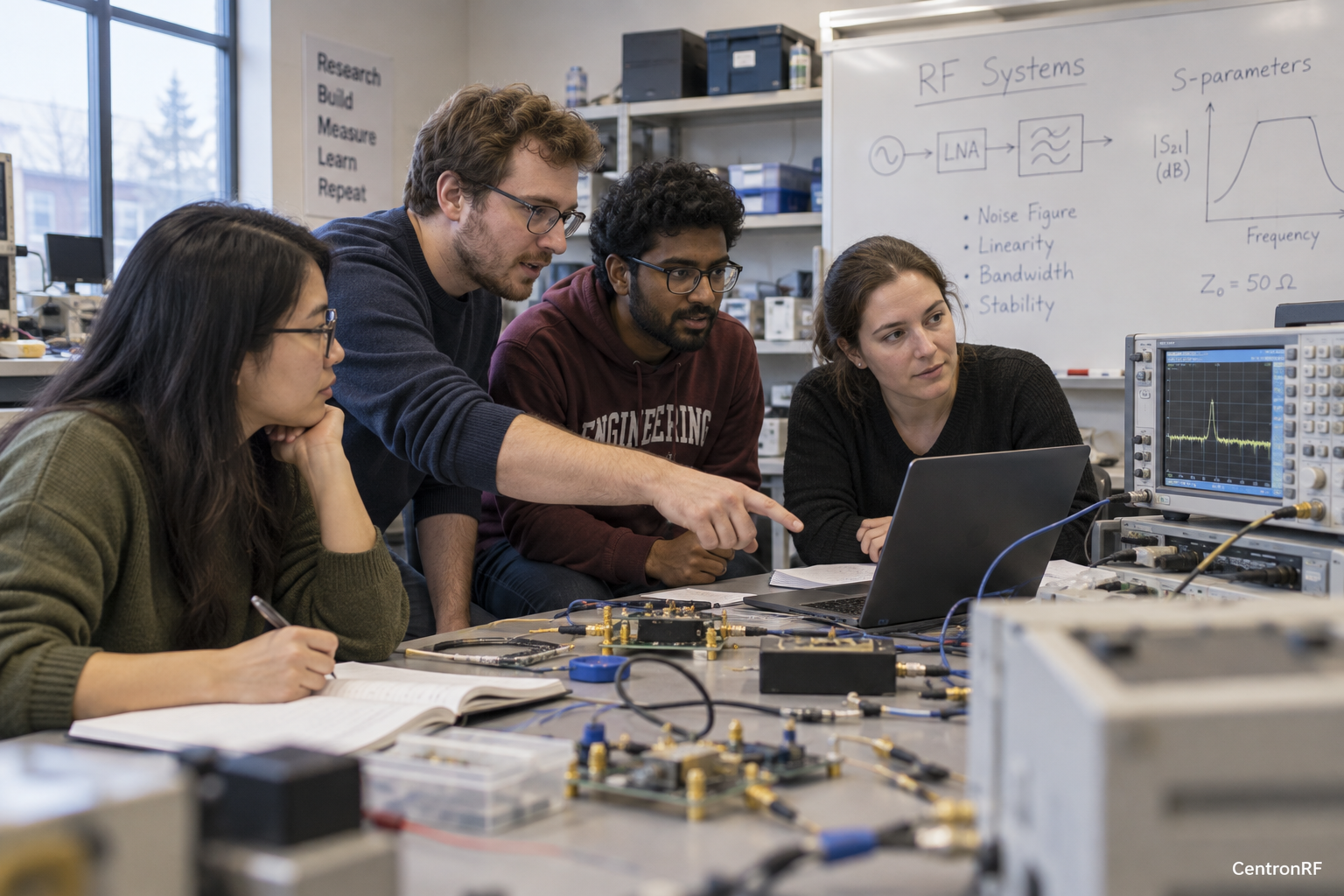
A noise-floor lesson demonstrates when a measurement becomes dominated by the setup's noise rather than the intended signal.
Why this matters in the industry
Students need to understand why displayed numbers at very low levels may not support the desired conclusion.
The technical reasoning
A noise floor limits the smallest quantity that a measurement method can resolve under defined settings. Averaging, bandwidth and input loss change the observed floor and the useful dynamic range. A result close to the floor should not be treated as an exact signal value or proof of absence.
Loss, noise and the position of the first active stage
The effect of loss depends on where it occurs. A passive loss before a low-noise amplifier reduces the wanted signal and adds thermal noise according to its temperature. Under the standard matched model, a passive network at the reference temperature has noise factor equal to its linear loss. In a cascade, later-stage noise contributions are divided by the gains preceding them, so moving the same loss to another position can change the overall noise figure.
How to structure the investigation
Use a suitable low-level source and qualified route. Compare observations under documented instrument settings and background conditions. Record the usable signal range and explain how bandwidth and averaging choices affect interpretation within the instrument's method.
Draw the sequence of passive and active stages and state the temperatures and reference conditions used by the model. Work in linear factors for cascade calculations, then convert to dB for reporting. Distinguish noise figure from receiver sensitivity, which additionally depends on bandwidth, waveform and the required detection or error criterion. Check that a sensitivity experiment is not limited by source leakage or the measurement setup.
Worked example or engineering scenario
Reducing an ideal white-noise measurement bandwidth by a factor of ten reduces integrated noise power by about 10 dB. The bandwidth change also alters what signal behavior the measurement captures.
Evidence to collect
| Record | Purpose |
|---|---|
| Instrument settings | Defines the tested state and scope of the comparison. |
| Background observation | Makes the stimulus or route condition reproducible. |
| Usable range | Supports interpretation of variation and possible confounding effects. |
| Averaging method | Connects the observation with the stated engineering decision. |
Trade-offs and common interpretation errors
Do not apply a simple room-temperature approximation to a different thermal condition without review. A power correction may reconstruct a signal level but cannot undo the signal-to-noise degradation caused by preceding loss. Keep estimates separate from measured noise performance and state the assumptions behind either result.
What the result can support
State measurement bandwidth and floor conditions and use appropriate limits when a signal is not resolved.
A low displayed value does not necessarily represent a resolved DUT signal.
Further technical reading
Related industry knowledge
- How to Use RF Loads in Network Analyzer Exercises
- How to Teach RF Link Budgets with a Conducted Setup
Numerical scenarios are illustrative assumptions, not reported measurements of a supplied product or installation.