


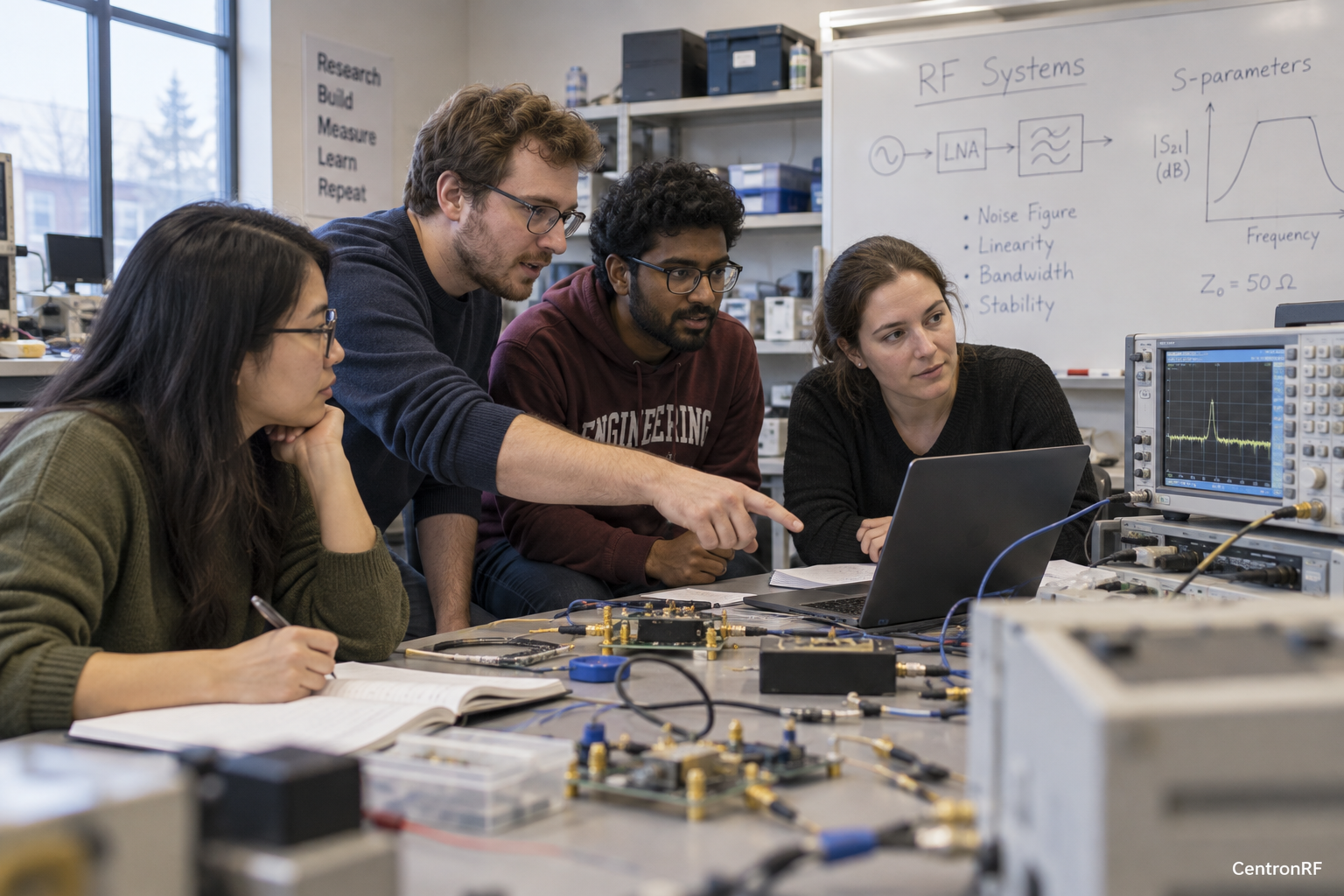
Cable-loss demonstrations compare a defined RF route with a suitable reference over the frequencies of interest.
Why this matters in the industry
Teaching labs can use the experiment to show why connection hardware becomes part of the measurement.
The technical reasoning
A cable-loss demonstration introduces frequency-dependent transfer, connector repeatability and the distinction between a nominal route and a measured one. Students should first control source and instrument conditions, then vary only the route. Repeating the complete connection process reveals variability that repeated readings from a single connection may miss.
From instrument readings to defensible results
Calibration, correction and verification have different roles. Calibration establishes a relationship under stated conditions; correction uses a model to adjust an indication; verification checks selected behavior against a defined criterion. A calibrated instrument does not automatically characterize the cables, adapters, fixtures and software around it. Repeated readings can estimate some random variation, but they do not expose every systematic error. The method must identify the measured quantity and the route through which its value is inferred.
How to structure the investigation
Calibrate or characterize the measurement setup appropriately. Sweep the cable route, record connector and adapter identities, and compare different frequencies. Keep routing and connection conditions repeatable so students can separate frequency effects from setup changes.
Define the plane, frequency range and operating state. Preserve raw readings, correction files and reference identities, and distinguish measurements made without reconnecting from repetitions of the full setup. Use an independent reference check where practical. When comparing two routes or stations, collect repeated observations and look for frequency-dependent offsets and spread. Investigate unexplained differences before treating a software correction as a solution.
Worked example or engineering scenario
A cable loses 0.5 dB at one frequency and 1.8 dB at another. The source level can be unchanged while the received level differs because the route response changes with frequency.
Evidence to collect
| Record | Purpose |
|---|---|
| Frequency sweep | Defines the tested state and scope of the comparison. |
| Cable identity | Makes the stimulus or route condition reproducible. |
| Adapters | Supports interpretation of variation and possible confounding effects. |
| Connection repeatability | Connects the observation with the stated engineering decision. |
Trade-offs and common interpretation errors
Agreement between two systems can conceal a shared error. A stable reference can also drift or be damaged. State the scope of the comparison and the evidence supporting the reference's stability. A small observed difference should be interpreted alongside uncertainty and repeatability, rather than assumed to be a meaningful device improvement.
What the result can support
Have students retain raw readings and compare both frequency dependence and reconnection variability.
A single low-frequency reading does not characterize the entire cable operating band.
Further technical reading
Related industry knowledge
- Energy Absorption and Reflection in an RF Teaching Experiment
- How to Build a Simple RF Attenuation Experiment
Numerical scenarios are illustrative assumptions, not reported measurements of a supplied product or installation.